03. Quantitative Data Charts in Notebooks
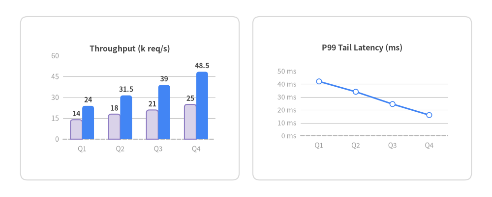
Drawlib includes 10 quantitative chart components (BarChart, LineChart, AreaChart, PieChart, RadarChart, BoxChart, ScatterChart, GanttChart, HeatmapChart, HeatmapOverlay) that sit alongside callouts, icons, and architecture diagrams on a single canvas.
View Drawlib Python Code
from drawlib.canvas import save, setup
from drawlib.charts.bar import BarChart
from drawlib.charts.line import LineChart
from drawlib.shapes import rectangle
from drawlib.styles import Colors, Styles

setup(width=144, height=58)

card_bg = Styles.White.patch(shape_r=2.0, shape_line_color=Colors.Gray3)
rectangle((38.0, 29.0), width=64.0, height=48.0, style=card_bg)
rectangle((106.0, 29.0), width=64.0, height=48.0, style=card_bg)

bar = BarChart(
    axis_line_style=Styles.MutedDashed,
    categories=["Q1", "Q2", "Q3", "Q4"],
    width=56.0,
    height=34.0,
    bar_mode="group",
    bar_width_ratio=0.62,
    bar_r=0.8,
    axis_text_style=Styles.Muted.patch(text_size=10.0),
    grid_style=Styles.MutedThin,
    value_text_style=Styles.DarkBold.patch(text_size=10.0),
    value_format="{:.1f}",
    title="Throughput (k req/s)",
    title_style=Styles.DarkBold.patch(text_size=11.5),
)
bar.add_series("Baseline", [14.0, 18.0, 21.0, 25.0], style=Styles.SecondaryNeutral)
bar.add_series("Cached", [24.0, 31.5, 39.0, 48.5], style=Styles.PrimaryFlat)
bar.configure_y_axis(min_value=0.0, max_value=60.0, tick_step=15.0)
bar.draw(xy=(10.0, 12.0))

line_chart = LineChart(
    axis_line_style=Styles.MutedDashed,
    categories=["Q1", "Q2", "Q3", "Q4"],
    width=56.0,
    height=34.0,
    show_points=True,
    point_size=0.75,
    axis_text_style=Styles.Muted.patch(text_size=10.0),
    grid_style=Styles.MutedThin,
    title="P99 Tail Latency (ms)",
    title_style=Styles.DarkBold.patch(text_size=11.5),
)
line_chart.add_series("P99 (ms)", [42.0, 34.0, 24.5, 16.0], style=Styles.PrimaryFlat, line_width=2.2)
line_chart.configure_y_axis(min_value=0.0, max_value=50.0, tick_step=10.0, format="{:.0f}", unit="ms")
line_chart.draw(xy=(78.0, 12.0))

save()
1. Computing Metrics in Python Cells
Because notebook cells share state, you can aggregate or transform data in standard Python cells before passing the series into a Drawlib chart:
In [setup]:
!pip install -q drawlib
In [1]:
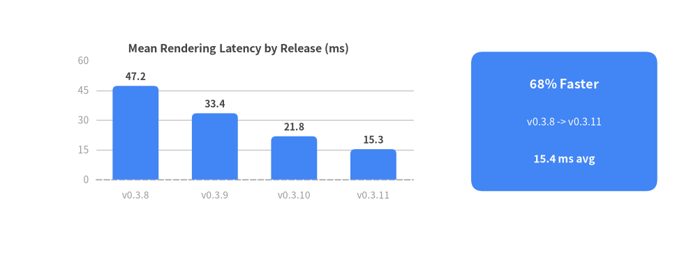
raw_latencies_ms = {
    "v0.3.8": [48.2, 46.0, 49.5, 45.1],
    "v0.3.9": [34.0, 32.5, 35.1, 31.8],
    "v0.3.10": [22.4, 21.0, 23.1, 20.5],
    "v0.3.11": [15.8, 14.9, 16.2, 14.5],
}

releases = list(raw_latencies_ms.keys())
mean_latencies = [round(sum(vals) / len(vals), 1) for vals in raw_latencies_ms.values()]
for rel, avg in zip(releases, mean_latencies, strict=True):
    print(f"{rel}: mean={avg:.1f} ms")
mean_latencies
Out [1]:
v0.3.8: mean=47.2 ms
v0.3.9: mean=33.4 ms
v0.3.10: mean=21.8 ms
v0.3.11: mean=15.3 ms
[47.2, 33.4, 21.8, 15.3]
2. Plotting Computed Series with Annotation Cards
Remember that all Charts use a Bottom-Left (x0, y0) coordinate anchor:
In [2]:
from drawlib.canvas import show, setup
from drawlib.charts.bar import BarChart
from drawlib.shapes import rectangle
from drawlib.styles import Styles
from drawlib.text import text

setup(width=120, height=44, cwd=True)

chart = BarChart(
    axis_line_style=Styles.MutedDashed,
    categories=releases,
    width=66.0,
    height=30.0,
    bar_width_ratio=0.58,
    bar_r=0.8,
    axis_text_style=Styles.Muted.patch(text_size=10.0),
    grid_style=Styles.MutedThin,
    value_text_style=Styles.DarkBold.patch(text_size=10.0),
    value_format="{:.1f}",
    title="Mean Rendering Latency by Release (ms)",
    title_style=Styles.DarkBold.patch(text_size=11.5),
)
chart.add_series("Mean Latency", mean_latencies, style=Styles.PrimaryFlat)
chart.configure_y_axis(min_value=0.0, max_value=60.0, tick_step=15.0)
chart.draw(xy=(8.0, 8.0))

# Summary Callout Card on the Right (Center Anchor)
rectangle((97.0, 23.0), width=32.0, height=24.0, style=Styles.PrimaryFlat.patch(shape_r=2.0))
text((97.0, 29.5), "68% Faster", style=Styles.WhiteBold.patch(text_size=13))
text((97.0, 23.0), "v0.3.8 -> v0.3.11", style=Styles.White.patch(text_size=10.5))
text((97.0, 16.5), "15.4 ms avg", style=Styles.WhiteBold.patch(text_size=11))

show()
Out [2]: