BoxChart: 箱ひげ図・ストリッププロット・ハイブリッド重ね描き
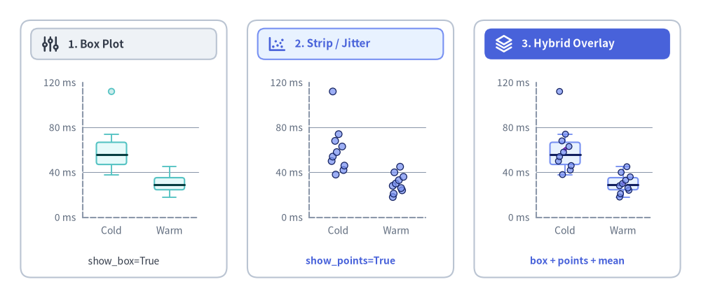
BoxChart(drawlib.charts.box)は、カテゴリ別の数値分布・四分位数・ばらつき・テールレイテンシを、生データ配列または事前集計済みの BoxStats から箱ひげ図・ストリップ/ジッタープロット・ハイブリッド重ね描きの 3 モードで宣言的に可視化します。
Source Code
from drawlib.canvas import save, setup
from drawlib.charts.box import BoxChart
from drawlib.icons import phosphor
from drawlib.shapes import rectangle
from drawlib.styles import Colors, Styles
from drawlib.text import text

setup(width=136, height=58)

cold_ms = [38, 42, 46, 50, 54, 58, 63, 68, 74, 112]
warm_ms = [18, 21, 24, 26, 28, 30, 33, 36, 40, 45]

card_style = Styles.Neutral.patch(shape_r=2.0, shape_line_color=Colors.Gray4, shape_fill_color=Colors.White)
for cx in (24.0, 68.0, 112.0):
    rectangle((cx, 29.0), width=40.0, height=50.0, style=card_style)

# Card headers with Phosphor icons (2 neutral badges + 1 focal PrimaryFlat badge)
rectangle((24.0, 49.4), width=36.0, height=6.0, style=Styles.Neutral.patch(shape_r=1.4))
phosphor.sliders((9.8, 49.4), width=3.8, style=Styles.DarkBold)
text((13.2, 49.4), "1. Box Plot", style=Styles.DarkBold.patch(text_size=11.0, halign="left"))

rectangle((68.0, 49.4), width=36.0, height=6.0, style=Styles.PrimaryNeutral.patch(shape_r=1.4))
phosphor.chart_scatter((53.8, 49.4), width=3.8, style=Styles.PrimaryBold)
text((57.2, 49.4), "2. Strip / Jitter", style=Styles.PrimaryBold.patch(text_size=11.0, halign="left"))

rectangle((112.0, 49.4), width=36.0, height=6.0, style=Styles.PrimaryFlat.patch(shape_r=1.4))
phosphor.stack((97.8, 49.4), width=3.8, style=Styles.WhiteBold)
text((101.2, 49.4), "3. Hybrid Overlay", style=Styles.WhiteBold.patch(text_size=11.0, halign="left"))

# 1. Left: Box Plot (show_box=True, show_points=False)
c_box = BoxChart(
    axis_line_style=Styles.MutedDashed,
    categories=["Cold", "Warm"],
    width=35.5,
    height=34.5,
    show_box=True,
    show_points=False,
    box_width_ratio=0.52,
    box_r=0.5,
    axis_text_style=Styles.Muted.patch(text_size=10.0),
    grid_style=Styles.MutedThin,
)
c_box.add_series("Latency", [cold_ms, warm_ms], style=Styles.SecondaryNeutral)
c_box.configure_y_axis(min_value=0, max_value=120, tick_step=40, unit="ms")
c_box.draw(xy=(6.5, 10.2))
text((24.0, 7.2), "show_box=True", style=Styles.Dark.patch(text_size=10.0))

# 2. Center: Strip / Jitter Plot (show_box=False, show_points=True)
c_strip = BoxChart(
    axis_line_style=Styles.MutedDashed,
    categories=["Cold", "Warm"],
    width=35.5,
    height=34.5,
    show_box=False,
    show_points=True,
    box_width_ratio=0.52,
    jitter=0.48,
    jitter_seed=42,
    point_radius=0.66,
    axis_text_style=Styles.Muted.patch(text_size=10.0),
    grid_style=Styles.MutedThin,
)
c_strip.add_series("Latency", [cold_ms, warm_ms], style=Styles.PrimaryNeutral)
c_strip.configure_y_axis(min_value=0, max_value=120, tick_step=40, unit="ms")
c_strip.draw(xy=(50.5, 10.2))
text((68.0, 7.2), "show_points=True", style=Styles.PrimaryBold.patch(text_size=10.0))

# 3. Right: Box + Strip Hybrid Overlay (show_box=True, show_points=True, show_mean=True)
c_hybrid = BoxChart(
    axis_line_style=Styles.MutedDashed,
    categories=["Cold", "Warm"],
    width=35.5,
    height=34.5,
    show_box=True,
    show_points=True,
    show_mean=True,
    box_width_ratio=0.52,
    box_r=0.5,
    jitter=0.48,
    jitter_seed=42,
    point_radius=0.58,
    axis_text_style=Styles.Muted.patch(text_size=10.0),
    grid_style=Styles.MutedThin,
)
c_hybrid.add_series(
    "Latency",
    [cold_ms, warm_ms],
    style=Styles.PrimaryNeutral,
    mean_style=Styles.AccentFlat.patch(shape_line_color=Colors.White, shape_line_width=1.1),
)
c_hybrid.configure_y_axis(min_value=0, max_value=120, tick_step=40, unit="ms")
c_hybrid.draw(xy=(94.5, 10.2))
text((112.0, 7.2), "box + points + mean", style=Styles.PrimaryBold.patch(text_size=10.0))

save()
1. 3 つの表示モード:箱ひげ・ストリップ・ハイブリッド重ね描き
従来のプロットライブラリでは箱ひげ図とジッター付きストリッププロットが別々のクラスに分かれていることが多いのに対し、BoxChart は show_box と show_points という 2 つの論理フラグ(チャート全体または add_series(...) の系列単位で指定可能)によって統計的な四分位要約と個別サンプル点を単一クラスに統合しています。
| 表示モード | show_box |
show_points |
描画内容と適したユースケース |
|---|---|---|---|
| 箱ひげ図(Box Plot) (デフォルト) | True |
False |
Q1〜Q3 の四分位箱、中央値ライン、T 字キャップ付きのひげ、および外れ値マーカー(show_outliers=True)を描画します。サンプル数が多い分布比較($N \ge 30$)や複数系列の並列比較に最適です。 |
| ストリップ/ジッタープロット | False |
True |
全サンプル点を決定論的な横方向ジッター(jitter=0.45、一直線に並べる場合は jitter=0.0)付きでプロットします。サンプル数が少なく($N < 15$)四分位箱だけでは偏りが見えにくい場合に有効です。 |
| ハイブリッド重ね描き(Box + Strip) | True |
True |
Q1〜Q3 の箱とひげの上に生の観測データ点を直接重ねて描画し、外れ値マーカーの二重描画を自動的に抑止します。$N = 5 \sim 30$ 程度のベンチマーク計測や PoC 評価に最適です。 |
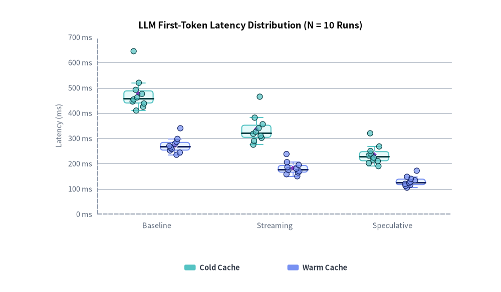
決定論的ジッターと平均値マーカー($N = 10$ ベンチマーク)
ストリップモードやハイブリッドモードで生データを描画する際、BoxChart は (jitter_seed, series_idx, category_idx) ごとに独立した 32 ビット素数ミキシングを用いてジッター変位を算出します。
- 100% Git 決定論的: 入力値と
jitter_seed=42が同じであれば、OS や Python プロセスを問わず常に完全に同一の座標にプロットされ、不要な画像差分が発生しません。 - アニメーション耐性: スライドの段階表示やアニメーションで一部の系列を非表示(
series.show = False)にしても、隣接する他系列のジッター配置が再シャッフルされることはありません。 - 算術平均マーカー(
show_mean=True): 中央値ラインと並べて高コントラストなひし形マーカー(mean_shape="rhombus")を描画できるため、テールレイテンシによって平均値が中央値から引き上げられている歪みを一目で把握できます。
from drawlib.canvas import save, setup
from drawlib.charts.box import BoxChart
from drawlib.styles import Colors, Styles

setup(width=106, height=62)

chart = BoxChart(
    axis_line_style=Styles.MutedDashed,
    categories=["Baseline", "Streaming", "Speculative"],
    width=92.0,
    height=48.0,
    show_box=True,
    show_points=True,
    show_mean=True,
    box_width_ratio=0.62,
    box_r=0.6,
    jitter=0.44,
    jitter_seed=42,
    point_radius=0.58,
    axis_text_style=Styles.Muted.patch(text_size=10.5),
    grid_style=Styles.MutedThin,
    title="LLM First-Token Latency Distribution (N = 10 Runs)",
    title_style=Styles.BlackBold.patch(text_size=13.0),
)

mean_badge = Styles.AccentFlat.patch(shape_line_color=Colors.White, shape_line_width=1.1)
chart.add_series(
    "Cold Cache",
    [
        [410, 425, 438, 446, 454, 462, 476, 492, 520, 645],
        [275, 290, 302, 310, 318, 326, 340, 356, 382, 465],
        [190, 202, 210, 216, 224, 232, 240, 250, 268, 320],
    ],
    style=Styles.SecondaryNeutral,
    mean_style=mean_badge,
)
chart.add_series(
    "Warm Cache",
    [
        [235, 244, 252, 258, 264, 270, 278, 286, 298, 340],
        [150, 158, 165, 170, 175, 180, 186, 195, 206, 238],
        [105, 112, 116, 120, 124, 128, 134, 140, 148, 172],
    ],
    style=Styles.PrimaryNeutral,
    mean_style=mean_badge,
)

chart.configure_y_axis(min_value=0, max_value=700, tick_step=100, unit="ms", label="Latency (ms)")
chart.draw(xy=(7.0, 11.0))
chart.draw_legend(
    xy=(39.0, 5.2),
    text_style=Styles.DarkBold.patch(text_size=10.5),
    orientation="horizontal",
    item_gap=6.0,
)

save()
2. ひげの算出モード(iqr・min_max・percentile)と外れ値制御
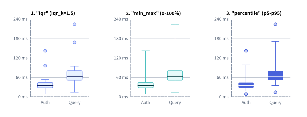
add_series(...) に生の数値シーケンス(Sequence[float])を渡すと、BoxChart は線形補間(inclusive 法)で四分位数(q1、median、q3)を算出し、whisker_mode に従って上下のひげ端点(min、max)および outliers を決定します。
whisker_mode="iqr"(デフォルト): 標準的な Tukey フェンス $[Q_1 - k \cdot \text{IQR},\ Q_3 + k \cdot \text{IQR}]$($\text{IQR} = Q_3 - Q_1$、デフォルトiqr_k=1.5)を適用します。ひげはフェンス内の最も外側の実測サンプル値まで伸び、フェンス外の値は個別の外れ値マーカー(show_outliers=True、outlier_shape="circle")として描画されます。whisker_mode="min_max": 観測サンプルの全範囲(0%〜100%:min(values)からmax(values))までひげを伸ばし、個別の外れ値マーカーは描画しません。whisker_mode="percentile":whisker_percentiles=(low_p, high_p)(デフォルト(5.0, 95.0)でp5〜p95、[q1, q3]を包含するようクランプ)にひげのキャップを配置し、そのパーセンタイル帯を超える上下の極端なスパイクを外れ値として分離します。
3 つのひげ算出モードの並列比較
以下の例では、8〜14 ms の高速キャッシュヒットから 224 ms のテールスパイクまでを含む同一の 20 サンプル API レイテンシデータを、0〜240 ms に揃えた Y 軸上で 3 種類の whisker_mode により並列比較しています。
from drawlib.canvas import save, setup
from drawlib.charts.box import BoxChart
from drawlib.styles import Styles

setup(width=136, height=52)

auth_ms = [8, 18, 22, 24, 26, 28, 29, 31, 32, 34, 35, 37, 39, 41, 43, 46, 49, 53, 96, 142]
query_ms = [14, 36, 42, 46, 49, 52, 55, 58, 60, 63, 65, 68, 72, 75, 79, 84, 88, 94, 168, 224]

configs = [
    ('1. "iqr" (iqr_k=1.5)', "iqr", Styles.PrimaryNeutral, 4.0),
    ('2. "min_max" (0-100%)', "min_max", Styles.SecondaryNeutral, 48.5),
    ('3. "percentile" (p5-p95)', "percentile", Styles.PrimaryFlat, 93.0),
]

for title, mode, series_style, x0 in configs:
    chart = BoxChart(
        axis_line_style=Styles.MutedDashed,
        categories=["Auth", "Query"],
        width=39.0,
        height=45.0,
        whisker_mode=mode,
        iqr_k=1.5,
        whisker_percentiles=(5.0, 95.0),
        box_width_ratio=0.52,
        cap_width_ratio=0.50,
        box_r=0.5,
        point_radius=0.65,
        outlier_shape="circle",
        axis_text_style=Styles.Muted.patch(text_size=10.0),
        grid_style=Styles.MutedThin,
        title=title,
        title_style=Styles.BlackBold.patch(text_size=11.0),
    )
    chart.add_series("API", [auth_ms, query_ms], style=series_style)
    chart.configure_y_axis(min_value=0, max_value=240, tick_step=60, unit="ms")
    chart.draw(xy=(x0, 3.5))

save()
3. 事前集計データ(BoxStats)と対数スケールによるテールレイテンシ可視化
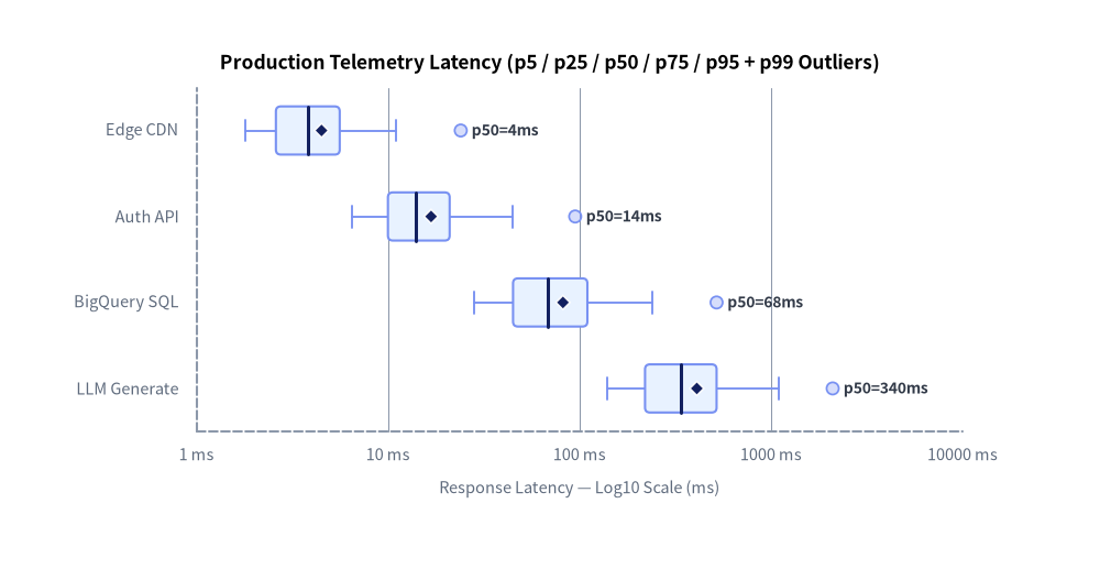
BigQuery(APPROX_QUANTILES)、Cloud Monitoring、Prometheus ヒストグラムなどの本番オブザーバビリティ基盤では、何百万件もの生リクエスト配列を取り出す代わりに、あらかじめ集計された分位点サマリ(p5、p25、p50、p75、p95、mean、p99 スパイクなど)を出力するのが一般的です。
BoxChart では BoxStats インスタンスを add_series(...) に直接渡すことができます(BoxStats、生データ配列 Sequence[float]、欠損スロット用の None/[] の混在にも対応)。さらに、2 ms のエッジ CDN から 1,500 ms 超の LLM 推論まで複数桁にまたがるレイテンシ分布では、orientation="horizontal" と常用対数軸 configure_x_axis(scale="log", ...) を組み合わせることで全サービス層を一枚のチャートで鮮明に比較できます。
from drawlib.canvas import save, setup
from drawlib.charts.box import BoxChart, BoxStats
from drawlib.styles import Styles

setup(width=112, height=58)

chart = BoxChart(
    axis_line_style=Styles.MutedDashed,
    categories=["Edge CDN", "Auth API", "BigQuery SQL", "LLM Generate"],
    orientation="horizontal",
    width=98.0,
    height=49.5,
    show_mean=True,
    box_width_ratio=0.56,
    box_r=0.5,
    point_radius=0.62,
    axis_text_style=Styles.Muted.patch(text_size=10.5),
    grid_style=Styles.MutedThin,
    value_text_style=Styles.DarkBold.patch(text_size=10.0),
    value_format="p50={:.0f}ms",
    title="Production Telemetry Latency (p5 / p25 / p50 / p75 / p95 + p99 Outliers)",
    title_style=Styles.BlackBold.patch(text_size=12.5),
)

chart.add_series(
    "Prod SLA",
    [
        BoxStats(min=1.8, q1=2.6, median=3.8, q3=5.6, max=11.0, mean=4.5, outliers=[24.0]),
        BoxStats(min=6.5, q1=10.0, median=14.0, q3=21.0, max=45.0, mean=16.8, outliers=[95.0]),
        BoxStats(min=28.0, q1=45.0, median=68.0, q3=110.0, max=240.0, mean=82.0, outliers=[520.0]),
        BoxStats(min=140.0, q1=220.0, median=340.0, q3=520.0, max=1100.0, mean=410.0, outliers=[2100.0]),
    ],
    style=Styles.PrimaryNeutral,
)

chart.configure_x_axis(
    scale="log",
    min_value=1,
    max_value=10000,
    ticks=[1, 10, 100, 1000, 10000],
    unit="ms",
    label="Response Latency — Log10 Scale (ms)",
)
chart.draw(xy=(7.0, 4.5))

save()
4. コンストラクタ・メソッド・データモデルのリファレンス
BoxChart コンストラクタ
BoxChart のコンストラクタ引数はすべてキーワード専用引数(*)です。
from drawlib.charts.box import (
    Axis,
    BoxChart,
    BoxStats,
    DrawDirection,
    FormatterType,
    LegendPosition,
    Orientation,
    PointShape,
    ScaleType,
    Series,
    WhiskerMode,
)
| パラメータ | 型 | デフォルト | 説明 |
|---|---|---|---|
axis_line_style |
Style |
必須 | 直交座標ベースラインのストロークに用いる必須アンカースタイル。 |
width / height |
float |
68.0 / 44.0 |
キャンバス上でのチャート全体のバウンディングコンテナ寸法(> 0.0)。 |
categories |
list[str] | None |
None |
カテゴリ軸に沿った順序付きカテゴリ名リスト。 |
orientation |
Orientation |
"vertical" |
"vertical"(X 軸がカテゴリ、Y 軸が数値)または "horizontal"(Y 軸がカテゴリ、X 軸が数値)。 |
show_box |
bool |
True |
Q1〜Q3 箱・ひげ・T 字キャップ・中央値ラインのデフォルト表示フラグ。 |
show_points |
bool |
False |
ジッター付きストリップ点のデフォルト表示フラグ(show_box と show_points の少なくとも一方は True が必須)。 |
show_outliers |
bool |
True |
show_box=True かつ show_points=False のときに外れ値マーカーを描画するかどうか。 |
show_mean |
bool |
False |
算術平均マーカーのデフォルト表示フラグ。 |
whisker_mode |
WhiskerMode |
"iqr" |
生データ配列に対するひげ算出ルール("iqr"、"min_max"、"percentile")。 |
iqr_k |
float |
1.5 |
whisker_mode="iqr" 時に IQR へ掛ける非負のフェンス係数。 |
whisker_percentiles |
tuple[float, float] |
(5.0, 95.0) |
whisker_mode="percentile" 時の下限・上限パーセンタイル (low_p, high_p)(0.0 <= low < high <= 100.0)。 |
box_width_ratio |
float |
0.65 |
各カテゴリスロットのうち箱クラスタ全体が占める幅の比率((0.0, 1.0])。 |
cap_width_ratio |
float |
0.45 |
個々の箱の幅に対するひげ先端 T 字キャップの長さ比率([0.0, 1.0]、0.0 でキャップ非表示)。 |
box_r |
float |
0.0 |
Q1〜Q3 箱の四隅に適用する角丸半径(>= 0.0)。 |
jitter |
float |
0.45 |
ストリップ点の横方向(または縦方向)への正規化拡散幅([0.0, 1.0]、0.0 で中心線上に整列)。 |
jitter_seed |
int |
42 |
スロット別の素数ミキシングに用いる決定論的ジッターシード整数。 |
point_radius |
float |
0.58 |
ストリップ点・外れ値・平均値マーカーのデフォルト半径(> 0.0)。 |
point_shape |
PointShape |
"circle" |
ストリップ点のデフォルト形状("circle"、"square"、"rhombus"、"triangle"、"none")。 |
outlier_shape |
PointShape |
"circle" |
外れ値マーカーの形状。 |
mean_shape |
PointShape |
"rhombus" |
算術平均マーカーの形状。 |
axis_text_style |
Style | None |
None |
目盛りラベル・カテゴリ名・軸タイトルのスタイル(None の場合は非表示)。 |
grid_style |
Style | None |
None |
背景の数値グリッド線のスタイル(None の場合は非表示)。 |
value_text_style |
Style | None |
None |
上端(または右端)の外側に描画される中央値ラベルのスタイル(None の場合は非表示)。 |
value_format |
FormatterType |
None |
中央値ラベル用のフォーマット文字列(例:"{:.1f}ms")または関数 Callable[[float], str]。 |
background_style |
Style | None |
None |
チャート外枠の背景カードのスタイル(None の場合は非表示)。 |
title / title_style |
str / Style | None |
"" / None |
チャート上部のタイトル文字列とタイポグラフィスタイル(描画には両方の指定が必要)。 |
系列登録・描画メソッド(add_series・draw・draw_legend)
| メソッド/プロパティ | シグネチャと主要引数 | 説明 |
|---|---|---|
add_series |
(name: str, data: Sequence[BoxStats | Sequence[float] | None], style: Style, legend_text_style: Style | None = None, *, show_box=None, show_points=None, show_outliers=None, show_mean=None, median_style=None, whisker_style=None, point_style=None, outlier_style=None, mean_style=None, point_radius=None, point_shape=None, jitter=None, show=True, draw_ratio=1.0, draw_direction=None) -> Series |
分布データ系列を登録し(個別指定がない限り style から高コントラストな中央値線・ひげ・マーカー色を自動導出)、変更可能な Series を返します。 |
configure_x_axis / configure_y_axis |
(scale=None, min_value=None, max_value=None, ticks=None, tick_step=None, format=None, unit=None, label=None, show_grid=None, grid_style=None, show_axis_line=None, line_style=None, show_ticks=None, tick_label_style=None) -> Axis |
線形/対数("log")スケール、上下限、目盛り、単位、軸タイトルを設定します。詳細は 軸・スケール・凡例 を参照してください。 |
draw |
(xy: tuple[float, float] = (0.0, 0.0), *, width: float | None = None, height: float | None = None, align: Literal["bottom_left", "center"] = "bottom_left", scale: float = 1.0) -> None |
基準座標 xy(デフォルト "bottom_left" または "center")にチャートを描画します。一時的な寸法上書きや比例 scale にも対応しています。 |
draw_legend |
(xy: tuple[float, float], text_style: Style, orientation: Orientation = "vertical", swatch_width: float = 2.4, swatch_height: float = 1.2, item_gap: float = 4.0, *, scale: float = 1.0) -> None |
分離配置された系列凡例を任意の xy に描画します(軸・スケール・凡例 参照)。 |
get_size |
() -> tuple[float, float] |
チャートコンテナの (width, height) を返します。 |
value_axis / category_axis |
Axis (プロパティ) |
向きに応じた軸アクセサ。value_axis は縦向き時に y_axis、横向き時に x_axis を返します(series、x_axis、y_axis も参照可能)。 |
BoxStats データモデルとヘルパーメソッド
BoxStats は単調増加順序(min <= q1 <= median <= q3 <= max)を検証する厳格な Pydantic モデル(extra="forbid")です。
| フィールド/クラスメソッド | 型 | デフォルト | 説明 |
|---|---|---|---|
min |
float |
必須 | 下側ひげ端点(標本最小値、下側 Tukey フェンス、または p5 など)。 |
q1 |
float |
必須 | 第 1 四分位数(25 パーセンタイル)。 |
median |
float |
必須 | 中央値(50 パーセンタイル)。 |
q3 |
float |
必須 | 第 3 四分位数(75 パーセンタイル)。 |
max |
float |
必須 | 上側ひげ端点(標本最大値、上側 Tukey フェンス、または p95 など)。 |
mean |
float | None |
None |
show_mean=True 時に描画される任意の算術平均値。 |
outliers |
list[float] |
[] |
show_box=True かつ show_points=False 時に描画される [min, max] 外の外れ値リスト。 |
points |
list[float] |
[] |
show_points=True 時に描画される生サンプル値リスト(show_box=False, show_points=True 時は必須)。 |
BoxStats.from_values(...) |
(values: Sequence[float], *, whisker_mode: WhiskerMode = "iqr", iqr_k: float = 1.5, whisker_percentiles: tuple[float, float] = (5.0, 95.0)) -> BoxStats |
クラスメソッド | 生の数値シーケンスから mean・outliers・points を含む完全な BoxStats を算出します。 |
共通の軸フォーマット、対数目盛りのルール、複数チャートのキャンバス合成については Charts 概要 および 軸・スケール・凡例 を参照してください。